 Home
HomeWhat You Must Know About Weighted Linear Regression in R

The narrow path to machine learning (ML) leads through the rough terrain of the land of statistics. If you are striving to become a data specialist, then you could go deeper and learn the ABC’s of weighted linear regression in R (the programming language and the development environment). It’s helpful for organizing job interviews but also for solving some problems that enhance our quality in life.
To be able to handle ML and BI you need to make friends with regression equations. It’s not only enough to learn two or three methods and pass an exam. You’ve got to learn to solve the problems from daily life: to find dependency between variables; ideally, to be able to differentiate signal from noise.
To make a regression can be a piece of cake. The use of a basic model of <- y~x would suffice. The issue is how to make the model more accurate? Let’s imagine your model gave adjusted R squared (R2)= 0,867; how can you optimize it? Read on to find the answer.
Digesting the pie of regression
Regression is a parametrical tool utilized to predict the dependent variable when independent variables are introduced. It’s called parametric because certain presuppositions are made based on the data set. If the data set corresponds to these assumptions, regression yields great dividends.
However, if you are struggling to achieve greater accuracy, there is no need for panic. We’ll learn some tips on how to achieve more accurate results.
Mathematically, a linear regression is used to predict model (the dependent variable) presented as Y = βo + β1X + ∈
Where ∈ – Error
βo – Intercept (coefficient)
β1 – Slope (coefficient)
Y – Dependent variable
X – Independent variable
This equation is known as a simple linear regression. It’s linear since we have only one independent variable (x). In multiple regressions, we have very many independent variables. You might recall studying this equation at school.
Y – is what we try to predict
X – is a variable which we use to make a prediction
βo is the intercept. It’s the value you get when x=0.
β1 is the slope. It explicates the alterations in Y when X is diversified by one tiny unit.
∈ stands for the residual value, that is to say, it shows the discrepancy between the real and predicted values.
The error is part and parcel of our lives. We could choose the most robust algorithm, but there’ll always be an ∈, reminding us that we simply can’t predict the future precisely.
Squaring the ordinary least squares
Despite the fact that error is unavoidable; we can try to minimize it as much as possible. This technique is generally known as Ordinary Least Squares (OLS).
Linear regression gives an estimate that reduces the distance between the fitted line and all other data points. Practically speaking, OLS in regression optimizes the sum of all squared residuals.
Nowadays, with programming languages and free codes, you could do so much more! You could go beyond ordinary least squares to know more about different value. In R, when you plan on doing multiple linear regression with the help of ordinary least squares you need only one line of lm y x data code:
Model <- lm(Y ~ X, data = X_data).
X can be replaced by many other variables. This model can be used to predict from the new data set to add another line of code:
Y_pred <- predict(Model, data = new_X_data)
Generation of “perfect” data points
After that we can produce “perfect” data points for regression without any strain in R. Using lm y x data method we are able to garner the following results:
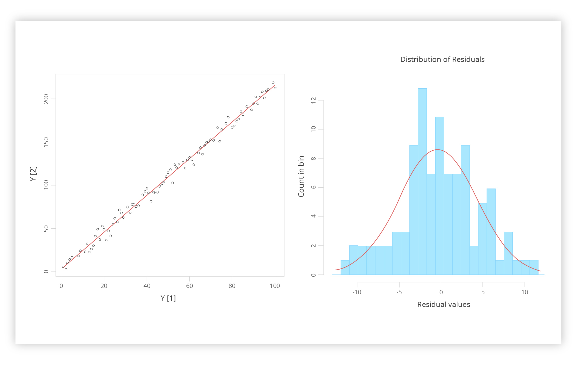
We have on the left the-so-called “noisy data.” The line here is a linear regression. On the right, we have a graph showing residuals. That’s the results of data points envisioned in the form of the histogram, where we can observe the curve of the same line. It helps us to see the superimposition of standard deviation. R provides us with a statistical model which gives an ideal summary. We get the following linear modeling:
> summary(Model)
Call:
     lm(formula =

Y_noisy ~ X, data = Y)
Residuals:
          Min 1Q

Median               3Q       Max
     -11.1348

-2.9799   0.3627

2.9478  10.3814
Coefficients:
                Estimate

Std. Error t value Pr(>|t|)
     (Intercept)

3.51543       0.98362

3.574 0.000548 ***
        X           2.11284          0.01691

124.946  < 2e-16 ***
---
     Signif. codes:

0 ‘***’ 0.001 ‘**’ 0.01 ‘*’ 0.05 ‘.’ 0.1 ‘ ’ 1
Residual standard error: 4.881 on 98 degrees of freedom
Multiple R-squared: 0.9938, Adjusted R-squared: 0.9937
     F-statistic:

1.561e+04 on 1 and 98 DF,  p-value: < 2.2e-16
We can see a slight deviation of coefficients from the underlying model. On top of that, both model parameter estimates are hugely crucial.
A more sophisticated plot
A more complex code looks like this:
X_data <- seq(1, 1000, 1)
#
# Y is linear in
x with uniform, periodic, and skewed noise
#
Y_raw
<- 1.37 + 2.097 * x
Y_noise
<- (X_data / 100) * 25 * (sin(2 * pi * X_data/100)) *
runif(n
= length(X_data), min = 3, max = 4.5) +
(X_data
/ 100)^3 * runif(n = 100, min = 1, max = 5)
Y
<- data.frame(X = X_data, Y = Y_raw + Y_noise)
We can get the following graphs via a prism of lm y x data
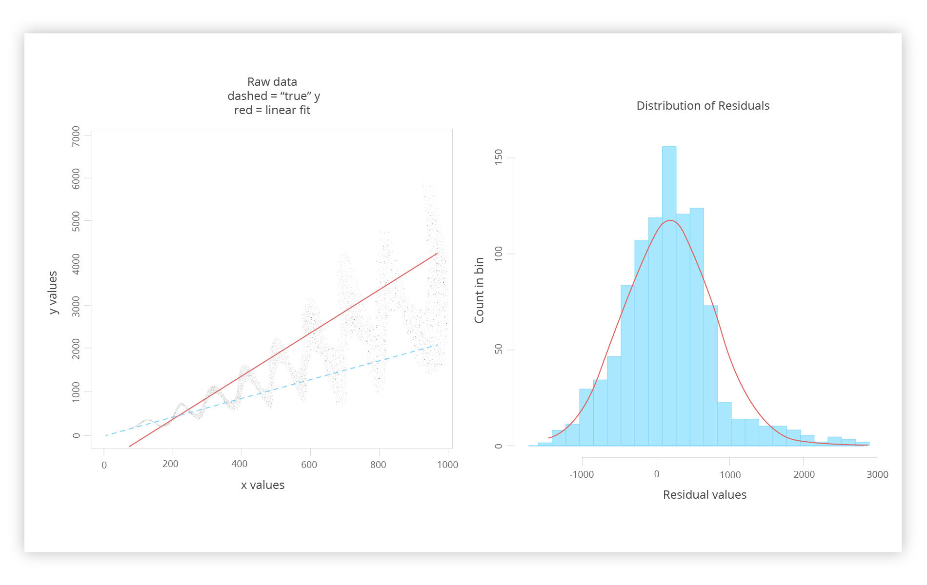
On the left, we see a graph of raw data, the red line represents the ordinary least squares line, and the dashed line depicts the “actual Y” which can still be an unknown variable. The right graph again shows the residual values and suggested remedy to improve the situation.
A disclaimer is needed here. First of all, this is quite an unrealistic scenario. If you didn’t know anything, imagine that the real Y was recurring at fixed intervals, amplified with X, assuming that the happening phenomena are most likely linear.
Let’s suppose that there’s a good reason for a good rationale for the existence of Y, considering the red line as too high. Taking all of it into consideration, you have to make your mind up as to what to do with all of these data points.
There’s always an option to sack the statistician who accumulated data with all of the standard errors and start from scratch again. For our purposes, let’s say you are launching some project tomorrow and you need to come up with a workable regression line to predict model for your control program.
A “noisy” graph
It just so happens that we have a lot of noise here. However, the residual chart to the right looks quite evenly distributed with all the squared residuals.
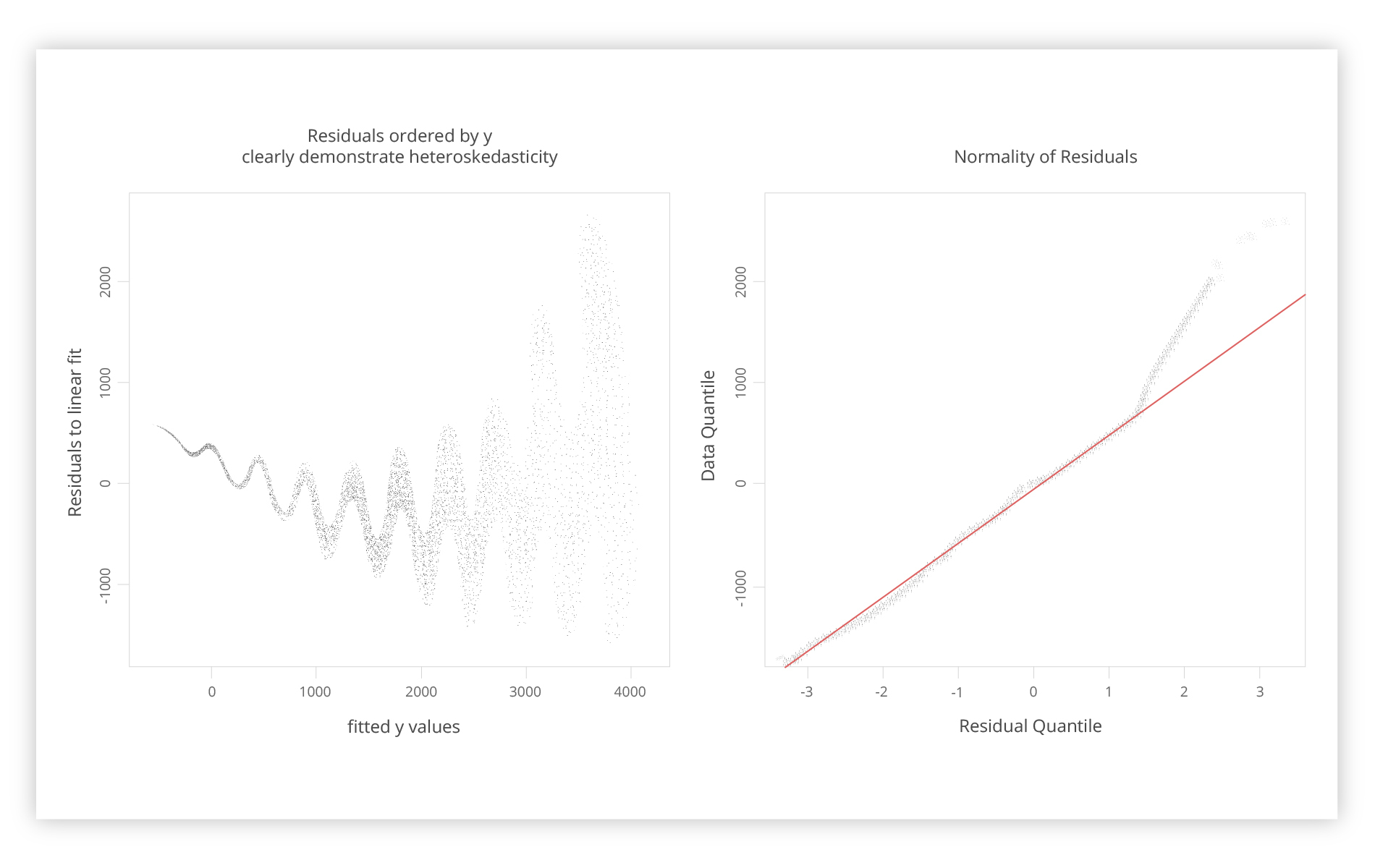
On the left is a representation of residual values versus the fitted Y values. The fundamental premise behind ordinary least squares is that the residuals aren’t dependent on the function’s value, and in this model, the residuals are equally distributed.
On the other hand, the left chart shows the disruption of this pattern. In fact, we are given more information here than in the left histogram. On the right is a typical Q-Q pattern which is modeled in such a way that residual values are all found on the red line. The higher you get, the more problematic it gets. So it’s indicative of what we could have missed if we had looked only at the histogram or the fit.
This type of behavior is called heteroscedasticity, which means the undesirable alterations on the part of residuals. What can be done about that? There are plenty of models, but for our case, we are going to pin down the weighted linear regression model.
A weighted linear regression model
Statistics as a science can be instrumental in a myriad of ways. For instance, it can assist in search of proper weights applicable to raw data points for making the regression model more accurate.
Typically, the “weights argument” works like this: to get the most plausible of the weights of the weighted linear model you need to divide the values of Y by the variance of residuals.
The hot potato question becomes: How do you get the variance values? The pragmatic answer is: A bin size in our case, 10 measurements, have to be defined.
Then a drifting value of the residual variance of 10 measurements in the bin can be calculated. This value can be used for the X that correlates to the bin center.
On the left and right spectrums of data in the weighted linear model, we’ve just used the discrepancy of the starting and the last 10 values accordingly. Voila, the value is now known for every Y value for the divergence of residuals.
Now we can use a robust linear regression that can be used with these weights:
Weighted_fit <- rlm (Y ~ X, data = Y, weights = 1/sd_variance)
Applying rlm, we get the following results:
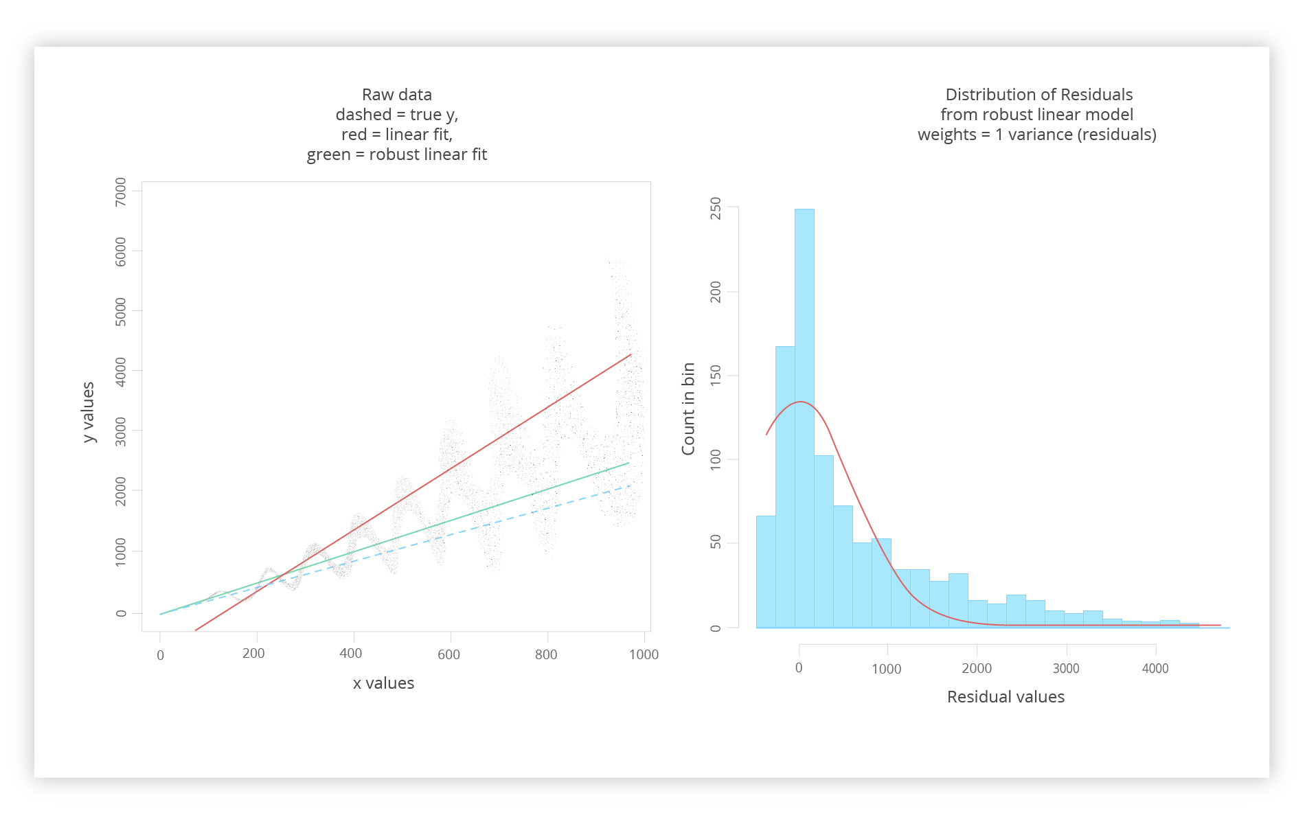
On the left, we see a new addition: a green line. Note that that the only new information that we get is residual variance. On the right, one can spot how twisted the residuals are.
Nonetheless, we are closer to the true Y.
Wrapping up:
The purpose of this article was to get you deeper into solving the regression problem. Sooner or later you’ll come across the issue of low model accuracy, and you’ll need to tackle it. Hopefully, you’ve got some insight into how to become more adept working with weighted linear regression in R.
Hopefully, you’ll know the importance of weighted least square in R for your future sales. The benefits of this technical process could save the day for your company if you know how to predict future trends more accurately.
Content created by our partner, Onix-systems.